Manually create a map index
This tutorial uses QGIS, a free and open-source GIS software application. Interested users can download the software from https://qgis.org/en/site/forusers/download.html.
In this section of the workflows for creating index maps, we will learn one way to manually create an index grid to facilitate spatially locating maps within a map series. Note that undertaking this task assumes there is no pre-existing grid created for the relevant series. If you have not already searched for this, it may be in your interest to do so before embarking on the following task–unless, of course, you are a GIS aficionado.
The Government of Canada makes available pre-made index maps for the National Topographic Series (NTS) at scales of 1:1m, 1:250k, and 1:50k. However, since various other NTS series exist at different scales (e.g., 1:500k, 1:125k), these pre-made indexes are hardly exhaustive. In these situations, we will need to adapt what already exists to suit our needs. In this example, we will modify the pre-existing Canada NTS 1:1m index map to create a 1:500k index.
For an introduction to the Canada NTS series, click here. For more information on the structure of the Canada NTS index, click here.
Import base index map to modify
Open QGIS and select New Empty Project.
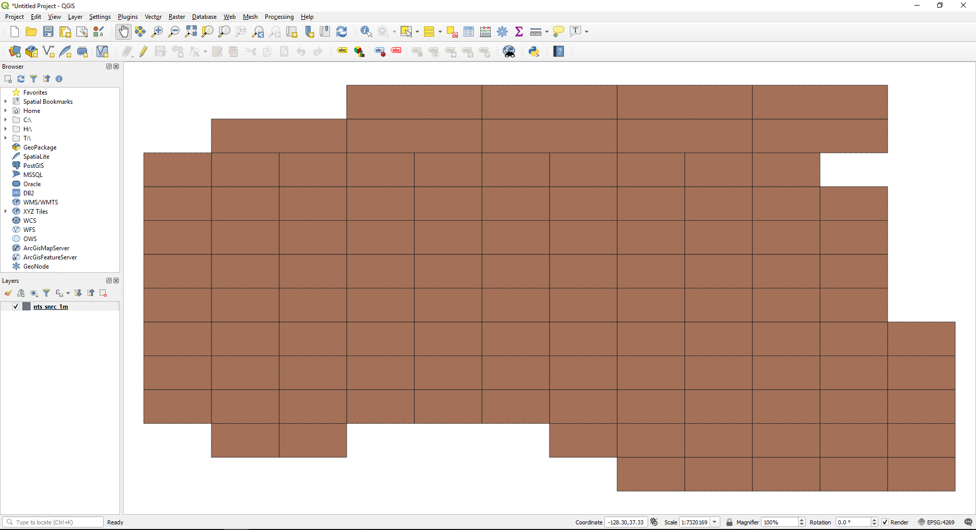
Open the location on your machine where you downloaded the original, base index map (in our case, the Canada NTS 1:1m index), click on the data file, and drag it into the Layers box in the lower left of the screen. (Note: User layout may vary.) Alternatively, you can import the layer by clicking Open Data Source Manager in the Data Source Manager Toolbar, or using the shortcut key Ctrl+L.
Select the appropriate transformation to the desired Coordinate Reference System (CRS) and click OK. In this example, we will use ‘EPSG:4326 - WGS 84’.
For an introduction to Coordinate Reference Systems, click here.
Your screen should look similar to this:
Set project CRS
To ensure a consistent CRS for all subsequent layers we create, we need to set the project CRS based on our layer CRS. To do this, click on the CRS icon in the bottom right of the screen.
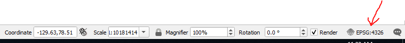
In the popup window, select the CRS you would like to use, click Apply, then OK. The CRS icon in the bottom right of the screen should now display the selected project CRS.
Creating grids
Next, we will create and overlay a spatial grid which subdivides each rectangular-polygon feature of the original, base layer into quarters. In order to run the algorithm, we must first determine:
- The extent of the geographic area of interest
- The horizontal and vertical spacing between the boundaries of features
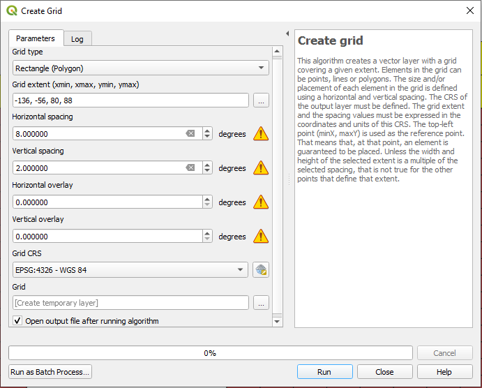
For our example, the geographic extent of Canada ranges from -48 to -144 degrees longitude and 40 to 88 degrees north latitude. While the vertical spacing will remain the same, at 2 degrees latitude, as a result of Canada’s far-northern extent, its horizontal spacing changes from 4 degrees longitude to 8 in the High Arctic (80 to 88 degrees north). This means we will have to create two grids–one from 40 to 80 degrees latitude, the other from 80 to 88–and merge them.
Create “southern” grid
First, we’ll create the “southern” grid. From the Menu Toolbar, select Processing > Toolbox > Vector creation > Create grid. The values you input should look like this:
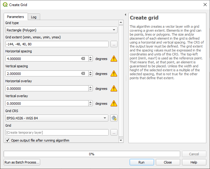
When you’ve entered the correct information, select Run, then Close. You should now see a grid covering all but Canada’s High Arctic.
If you intend to complete this task in more than one sitting, you will need to manually save each layer you create. Otherwise, they will not be present when you reopen the project, since they are created as temporary, or ‘scratch’, layers. (Fortunately, QGIS will notify you if you attempt to close a project with temporary layers.) To make a layer permanent:
1. Right-click on the layer
2. Select Make Permanent…
3. Choose the desired format and file name
4. Click OK
Improve visibility and verify extent
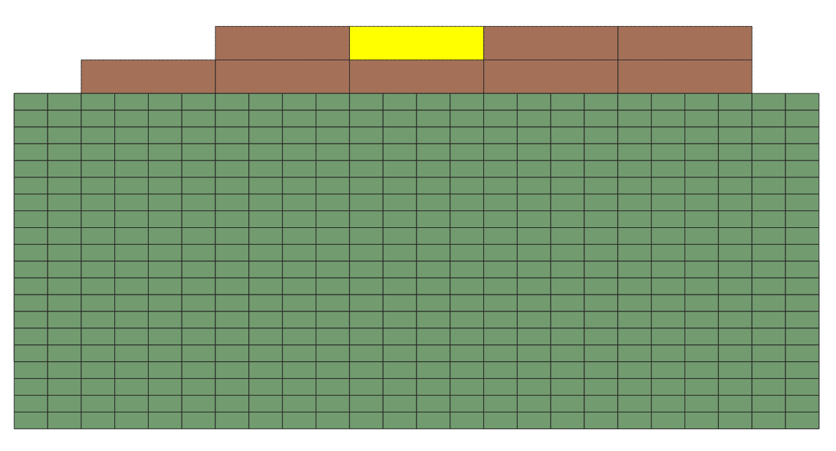
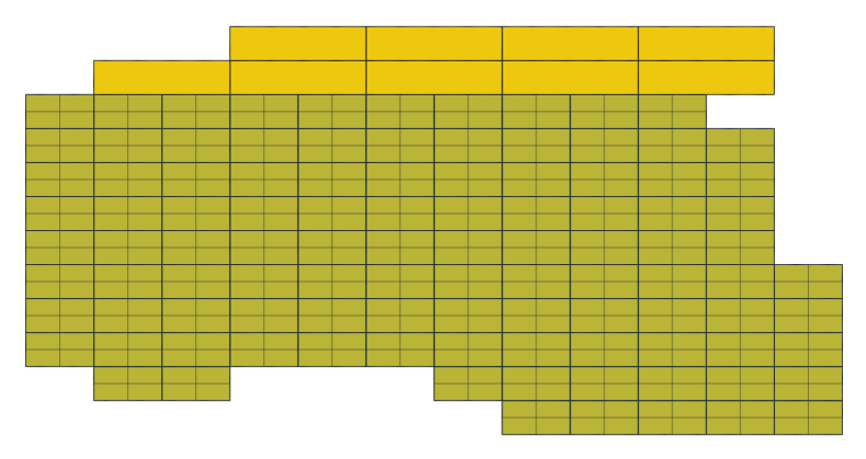
To make it easier to verify our grid matches the extent of the original, we’ll increase the transparency of our grid layer. Right-click the newly-created grid layer within the Layers box and select Properties… > Symbology. Adjust the layer’s opacity to, say, 25%. Click Apply, then OK. (You can also change the color combination of both layers for better visibility.)
![]()
We can now clearly see three things:
- Our grid matches the extent (N, S, E, W) we specified.
- The grid subdivides the rectangular polygons of the 1:1m index into quarters.
- There are features in our new grid that are not present in the original. (This is the result of the Create grid algorithm, which creates a rectangular grid that matches the input grid’s maximum N-S and E-W extent.)
Trim excess features
Since we only want to keep features that are present in both grids, we will have to remove those in the new grid which are not present in the old. To do this, click Select Features from the Selection Toolbar.
In the event you need to add a toolbar to your screen, select View > Toolbars and toggle on the desired one.
Select all the features on the new grid layer which do not overlap with the original. (Hold down the left-click button and drag the cursor over multiple features to select them. Press and hold the Shift key to select multiple segments.)
Once you’ve selected the non-overlapping features, right-click on the new grid layer in the Layers box and select Open Attribute Table. You should see some features highlighted in blue. Within the Attribute Table, in the top-left corner, click Toggle editing mode, then Delete selected features to the right. Click Save edits, Toggle editing mode, and close the Attribute-table popup window. Your screen should now look similar to this:
Rename layers
To help us mentally keep track of things as layers proliferate, rename the new layer by right-clicking on it in the Layers box and selecting Rename Layer. We will call it ‘south’, in reference to the ‘southern’ portion of the Canada grid we are creating, to contrast it with the ‘High Arctic’ portion we will create later. For added clarity, we will also rename the original layer to ‘original’.
From mere grid to mighty index: adding labels
Now that the outline of our grid matches the original, we want to transfer the NTS labels from the features of the original grid to the corresponding features of our new grid. To do this, we will make use of QGIS’ Join attributes by location algorithm. From the Menu Toolbar, select Processing > Toolbox > Vector general > Join attributes by location. Within the popup window, select the following three values:
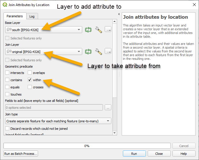
Click Run, then Close. Open the Attribute Table for the newly-created layer to verify it contains the attributes from both layers.
Rename the layer to ‘south_labels’. (‘labels’ indicates the layer contains the labels from the original NTS layer.)
Making each feature’s label unique
We now have the first portion of our label affixed to our grid’s features. However, since we subdivided the original grid’s features into quarters, we currently have four features in our new grid that share the same label from the original. Our next task, then, will be to add character strings to our labels, so we can uniquely identify each feature within the new grid. In this example, we will distinguish the features by appending either ‘SE’, ‘SW’, ‘NE’, or ‘NW’ to its label, depending on its relative position.
First, we will select all the south features for each label. To do this, click Select Features from the Attributes Toolbar. (Make sure you have the correct layer selected–“south_labels”, in our case.) Click on a feature in the bottom row of features with a shared label and drag the cursor to select the entire row across the grid. Press and hold Shift to continue this action, and select all of the south rows in the ‘south_labels’ layer. Your screen should look similar to this:
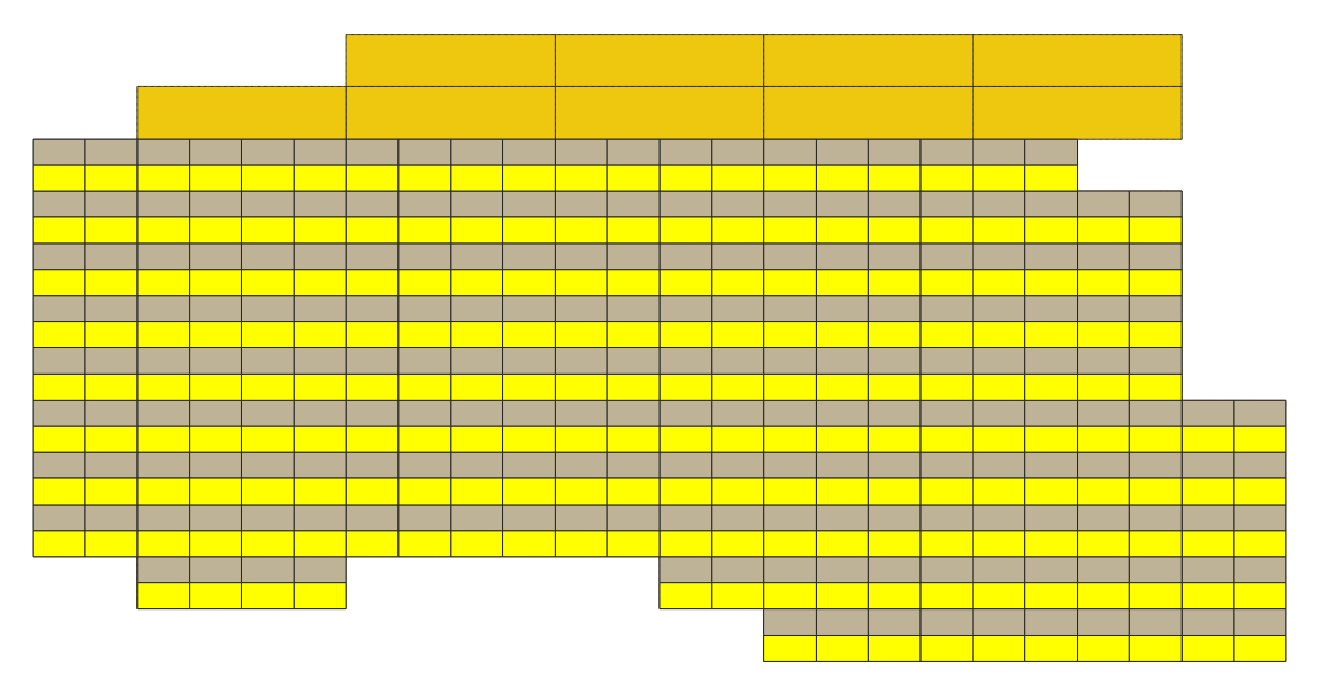
Open the Attribute Table for the ‘south_labels’ layer. You should now have half of the layer’s features selected–highlighted in blue–which you can verify by looking at the information on the top ribbon of the screen. Close the Attribute Table.
Select Processing > Toolbox > Vector table > Refactor fields. Input the displayed values in the following fields:
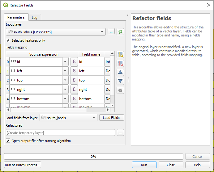
Make sure to click the Selected features only box. Failure to do so will add the ‘S’ character to every feature in the layer, rather than just the south features.
Before clicking Run on the Refactor Fields popup window, click the Expressions button for the “IDENTIF” field (the labels column):
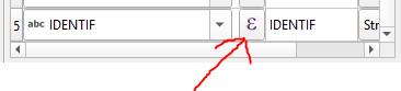
Within the Expression Dialog popup window, in the middle column, click String > rpad. Follow the documentation in the right column to create an expression in the left column that looks like this:
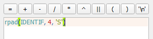
Click OK, then Run, and Close.
Rename the new refactored layer to something more descriptive. In our case, we’ll call it ‘south_labels_s’. (The ‘s’ denotes south features.)
Repeat this series of steps to create a layer for the north rows.
Merge layers
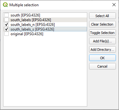
After we have both our south (‘south_labels_s’) and north (‘south_labels_n’) layers, we will merge them into a single layer. Click Processing > Toolbox > Vector general > Merge vector layers. From the Merge vector layers popup window, in the Input layers field, select the two layers you’d like to merge, and click OK.
Click Run, then Close. (The rest of the default settings are fine for our purposes.)
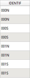
Open the Attribute Table and sort by the labels (‘IDENTIF’) column to verify the merge performed as expected. You should see two features sharing the same N/S label, as opposed to four after subdividing the original grid.
Rename the merged vector. (We’ll call it ‘south_labels_ns’.)
Repeat the previous steps (‘Making each feature’s label unique’ and ‘Merge layers’) on the ‘south_labels_ns’ layer for the ‘east’ and ‘west’ rows to derive the final layer for the ‘southern’ portion of our Canada grid.
High Arctic index
Now that we have unique labels for each feature of the ‘southern’ portion of our Canada grid, we’ll wrap up our project by creating another subdivided grid for the ‘High Arctic’ portion of the original grid. To do this, use the instructions above to repeat our earlier steps:
- Create a grid (See note below.)
- Trim excess features
- Transfer labels using Join attributes by location
- Use Refactor fields to create layers with ‘north’ and ‘south’ labels
- Merge ‘north’ and ‘south’ layers into a single layer
- Use this new merged ‘north-south’ layer to create layers with ‘east’ and ‘west’ labels
- Merge the ‘east’ and ‘west’ layers into a single ‘High Arctic’ layer
When creating the grid for Canada’s High Arctic, it’s important to keep in mind that the horizontal spacing will differ from the ‘southern’ grid–8 degrees, instead of 4. (If you remember from earlier, this is the reason we couldn’t create a single grid to begin with.)
Finished product
Once the ‘High Arctic’ layer is complete, merge it with the ‘southern’ layer to create the completed index. Don’t forget to make the layer permanent and save your project.
That’s it! You now have a digital map index that can be exported as a GeoJSON and associated with an OIM-compatible spreadsheet from the relevant paper-map collection. (See the ‘Create a virtual layer in QGIS’ lesson for more information.)